Introduction to Neural Networks
Applying CNNs
The MNIST data set is a collection of 70,000 28×28 pixel images of scanned, handwritten digits.
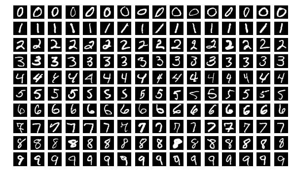
We want to create a network which can, given a similar image of a digit, identify its value.
Using TensorFlow to create and train a network
In TensorFlow, there are three main tasks needed before you can start training. You must:
- Specify the shape of your network
- Specify how the network should be trained
- Specify your training data set
We will now go through each of these to show how the parts fit together.
Designing the CNN
We will create a network which fits the following design:
- Convolutional Layer #1: Applies 16 5×5 filters (extracting 5×5-pixel subregions), with ReLU activation function
- Pooling Layer #1: Performs max pooling with a 2×2 filter and stride of 2 (which specifies that pooled regions do not overlap)
- Convolutional Layer #2: Applies 32 5×5 filters, with ReLU activation function
- Pooling Layer #2: Again, performs max pooling with a 2×2 filter and stride of 2
- Dense Layer #1: 128 neurons, with dropout regularization rate of 0.4 (probability of 40% that any given element will be dropped during training)
- Dense Layer #2 (Logits Layer): 10 neurons, one for each digit target class (0–9).
This structure has been designed and tweaked specifically for the problem of classifying the MNIST data, however in general it is a good starting point for any similar image classification problem.
Building the CNN
We're using TensorFlow to create our CNN but we're able to use the Keras API inside it to simplify the network construction. We build up our network sequentially, layer-by-layer.
First convolutional layer
We start with our first convolutional layer. It create 16 5×5 filters. Since we have specified padding="same", the size of the layer will still be 28×28 but as we specified 16 filters, the overall size of the layer will be 28×28×16=12,544.
import tensorflow as tf

model = tf.keras.models.Sequential([
    tf.keras.layers.Conv2D(
        filters=16,
        kernel_size=5,
        padding="same",
        activation=tf.nn.relu
    ),
])
First pooling layer
Next we add in a pooling layer. This reduces the size of the image by a factor of two in each direction (now effectively a 14×14 pixel image). This is important to reduce memory usage and to allow feature generalisation.
model = tf.keras.models.Sequential([
    tf.keras.layers.Conv2D(
        filters=16,
        kernel_size=5,
        padding="same",
        activation=tf.nn.relu
    ),
    # ↓ new lines ↓
    tf.keras.layers.MaxPool2D((2, 2), (2, 2), padding="same"),
])
After pooling, the layer size is 14×14×16=3136.
Second convolutional and pooling layers
We then add in our second convolution and pooling layers which reduce the image size while increasing the width of the network so we can describe more features:
model = tf.keras.models.Sequential([
    tf.keras.layers.Conv2D(
        filters=16,
        kernel_size=5,
        padding="same",
        activation=tf.nn.relu
    ),
    tf.keras.layers.MaxPool2D((2, 2), (2, 2), padding="same"),
    # ↓ new lines ↓
    tf.keras.layers.Conv2D(
        filters=32,
        kernel_size=5,
        padding="same",
        activation=tf.nn.relu
    ),
    tf.keras.layers.MaxPool2D((2, 2), (2, 2), padding="same"),
])
After this final convolution and pooling, we have a layer of size 7×7×32=1568.
Fully-connected section
Finally, we get to the fully-connected part of the network. At this point we no longer consider this an 'image' any more so we flatten our 3D layer into a linear set of nodes. We then add in a dense (fully-connected) layer with 128 neurons.
To avoid over-fitting, we apply dropout regularization to our dense layer which causes it to randomly ignore 40% of the nodes each training cycle (to help avoid overfitting) before adding in our final layer which has 10 neurons which we expect to relate to each of our 10 classes (the numbers 0-9):
model = tf.keras.models.Sequential([
    tf.keras.layers.Conv2D(
        filters=16,
        kernel_size=5,
        padding="same",
        activation=tf.nn.relu
    ),
    tf.keras.layers.MaxPool2D((2, 2), (2, 2), padding="same"),
    tf.keras.layers.Conv2D(
        filters=32,
        kernel_size=5,
        padding="same",
        activation=tf.nn.relu
    ),
    tf.keras.layers.MaxPool2D((2, 2), (2, 2), padding="same"),
    # ↓ new lines ↓
    tf.keras.layers.Flatten(),
    tf.keras.layers.Dense(128, activation="relu"),
    tf.keras.layers.Dropout(0.4),
    tf.keras.layers.Dense(10, activation="softmax")
])
Telling it how to train
To finalise our model we once more use sparse, categorical cross-entropy as the loss function:
model.compile(
    loss="sparse_categorical_crossentropy",
    metrics=["accuracy"],
)
Sparse categorical cross-entropy should be used when you have a classification problem and the labels being used are the index of the desired class.
Getting the data into Python
We've now finished designing our network so we can start getting our data into place. TensorFlow comes with a built-in loader for the MNIST dataset which has a pre-configured train/test split:
import tensorflow as tf
import tensorflow_datasets as tfds

ds_train, ds_test = tfds.load(
    "mnist",
    split=["train", "test"],
    as_supervised=True,
)
ds_train and ds_test are both sequences of 28×28×1 matrices containing the numbers 0-255. Each example also has a label associated with it which is a single integer scalar from 0-9.
ds_train.element_spec
Creating the training dataset
The first thing we need to do with our data is convert it from being in the range 0-255 to being in the range 0.0-1.0:
def normalize_img(image, label):
    return tf.cast(image, tf.float32) / 255., label

ds_train = ds_train.map(normalize_img)
Then we shuffle each complete input set and collect them into batches of 128:
ds_train = ds_train.shuffle(1000)
ds_train = ds_train.batch(128)
Creating the test dataset
In order for it to be a fair comparison, we need to do some of the same pre-processing to the test dataset too:
ds_test = ds_test.map(normalize_img)
ds_test = ds_test.batch(128)
Fitting the model to the data
At this point, we're all ready to go. We call the fit method on the model, passing in the training data, how long to run for and the test data set to use:
model.fit(
    ds_train,
    validation_data=ds_test,
    epochs=2,
)
Testing the model in the real world
Let's start by downloading some example image files:
from urllib.request import urlretrieve

for i in list(range(1,10)) + ["dog"]:
    urlretrieve(f"https://github.com/milliams/intro_deep_learning/raw/master/{i}.png", f"{i}.png")
Then, load them in and convert them to the same format as the data that we trained and validated on:
import numpy as np
from skimage.io import imread

images = []
for i in list(range(1,10)) + ["dog"]:
    images.append(np.array(imread(f"{i}.png")/255.0, dtype="float32"))
images = np.array(images)[:,:,:,np.newaxis]
images.shape
images is in the same shape as our training and validation data. It's a 4D array of 10 images each 28×28 pixels with one colour channel. We can pass it directly to the model.predict method:
probabilities = model.predict(images)
To summarise all the results:
truths = list(range(1, 10)) + ["dog"]

table = []
for truth, probs in zip(truths, probabilities):
    prediction = probs.argmax()
    if truth == 'dog':
        print(f"{truth}. CNN thinks it's a {prediction} ({probs[prediction]*100:.1f}%)")
    else:
        print(f"{truth} at {probs[truth]*100:4.1f}%. CNN thinks it's a {prediction} ({probs[prediction]*100:4.1f}%)")
    table.append((truth, probs))
Or, in table form:


You should see that 5 seem to have worked well maybe some others have the correct answer with a low probability but most are struggling.
Your results will likely be different but they will probably have the same strengths and weaknesses. Can you see why some have predicted well, and other have not?
Exercise
Are you able to improve on the performance, either on the validation data set (val_accuracy), or on the examples, by tweaking the design of the network?
Are you able to get equivalent performance with a simpler network (fewer filters, fewer convolutional layers, fewer dense neurons)? Do you get better performance with a more complex network?